
Tutorial: Anomaly Detection Solution
In this tutorial, we are going to show you how to build an anomaly detection solution to the vibration data collected from the bearing sensors of two motors step by step. The purpose is to monitor the sensor data continuously and identify any unusual patterns that might indicate motor wear, bearing failure, or other operational issues.
We are going to use an Isolation Forest model, a machine learning technique specifically designed to isolate anomalies by identifying data points that behave differently from the majority. The model processes the sensor data to detect deviations, enabling us to identify potential issues early and take corrective action before they result in equipment failure.
By running this anomaly detection model, we aim to improve the reliability and performance of the motors by predicting failures and scheduling maintenance more effectively. The objective is to calculate in real time the probability to encounter an anomaly on our motors. We would like also to have a unique solution to edit and maintain for all our similar motors.
Prerequisite
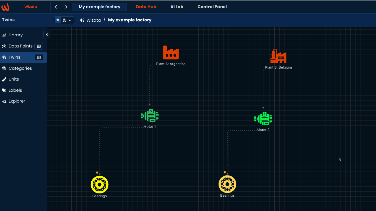
The tutorial focuses on a motor's digital twin, specifically its bearing component based on our sample data representing vibration sensors and associated digital twin.
Your environment should have the sample data flowing (mt1_bearing1, mt1_bearing2, ... mt2_bearing4) and your twin structure should look like with all sensors attached respectively to bearings on motor one and two:
If not already the case, please check the following articles to achieve those prerequisite.
- How to stream and loop the relevant sample data
- Follow how to creating and connecting Twin Units
Create a Template
The first step involves creating a Template with properties such as datapoints, JSON objects, floats, etc. The template helps organize everything in one place.
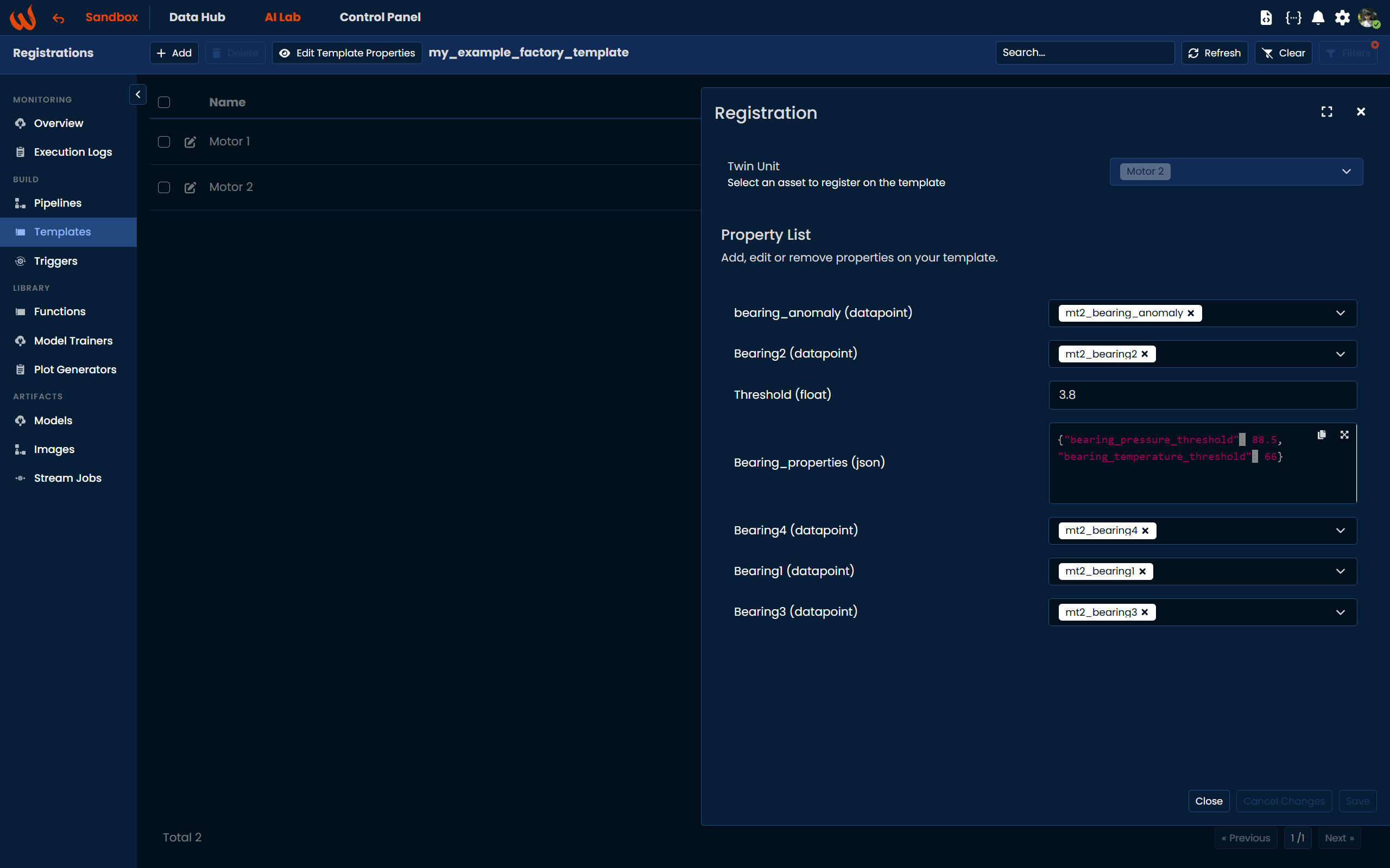
Since we have two motors to apply the anomaly detection model, the template allows us to use a single pipeline to apply the model to both motors efficiently. A template named "my_example_factory_template" could include the following:
- Datapoints: Bearing1, Bearing2, Bearing3, Bearing4, bearing_anomaly
- Variable: Threshold
- JSON: Bearing_properties
Using the Python Toolkit, you can register a template using the following logic:
wizata_dsapi.api().upsert_template(
    key="my_example_factory_template",
    name="My Example Factory Template"
)

wizata_dsapi.api().add_template_property(
    template='my_example_factory_template',
    property_name='Bearing1'
)

wizata_dsapi.api().add_template_property(
    template='my_example_factory_template',
    property_name='Bearing2'
)

wizata_dsapi.api().add_template_property(
    template='my_example_factory_template',
    property_name='Bearing3'
)

wizata_dsapi.api().add_template_property(
    template='my_example_factory_template',
    property_name='Bearing4',
    property_type='datapoint'
)

wizata_dsapi.api().add_template_property(
    template='my_example_factory_template',
    property_name='bearing_anomaly',
    property_type='datapoint'
)

wizata_dsapi.api().add_template_property(
    template='my_example_factory_template',
    property_name='Threshold',
    property_type='float'
)

wizata_dsapi.api().add_template_property(
    template='my_example_factory_template',
    property_name='Bearing_properties',
    property_type='json'
)
For anomaly detection model we have to create a logical datapoint as "mt1_bearing_anomaly", before registering the twin we should have that datapoint in the platform then we can map it:
datapoint = wizata_dsapi.DataPoint( hardware_id="mt1_bearing_anomaly",name="mt1_bearing_anomaly")
wizata_dsapi.api().create(datapoint)
Once your template is created, the next step is to register a Twin. Each asset will have fixed values for variables and/or mapped datapoints. When querying a registered Twin based on a template, there is no need to know the specific details of each datapoint.
To register the Twin, you must create a mapping between the template property names and their corresponding values:
wizata_dsapi.api().register_twin(
    template="my_example_factory_template",
    twin="motor_1",
    properties={
        "Bearing1": "mt1_bearing1",
        "Bearing2": "mt1_bearing2",
        "Bearing3": "mt1_bearing3",
        "Bearing4": "mt1_bearing4",
        "bearing_anomaly":"mt1_bearing_anomaly",
        "Threshold": 3.1,
        "Bearing_properties": {"bearing_pressure_threshold": 89.5,
                               "bearing_temperature_threshold": 67}

    }
)
We should apply the same registering twin for motor two as well.
wizata_dsapi.api().register_twin(
    template="my_example_factory_template",
    twin="motor_2",
    properties={
        "Bearing1": "mt2_bearing1",
        "Bearing2": "mt2_bearing2",
        "Bearing3": "mt2_bearing3",
        "Bearing4": "mt2_bearing4",
        "bearing_anomaly":"mt2_bearing_anomaly",
        "Threshold": 3.8,
        "Bearing_properties": {"bearing_pressure_threshold": 88.5,
                               "bearing_temperature_threshold": 66}

    }
)
We can create a template directly from the UI. Please see this article to create a Template from the UI
At the end of this process, we have a template that includes two Digital Twins: Motor 1and Motor 2, as shown below:
Create a Pipeline
After creating the template, the next step is to develop a Pipeline to integrate the solution. A pipeline consists of a series of steps necessary for the project, including querying, transformation, machine learning (ML) models, plots, and writing results.
Using the Python Toolkit, you can create a pipeline programmatically as follows:
import uuid
# Generate pipeline
pipeline = wizata_dsapi.Pipeline(  # create a pipeline
    key="bearing_anomaly_pipeline",
    template_id=uuid.UUID("61d63f8b-6142-43bc-bb98-ac146076601b") # this template id is important and it's coming from the template link
    # the end of the link is giving us the template id
)
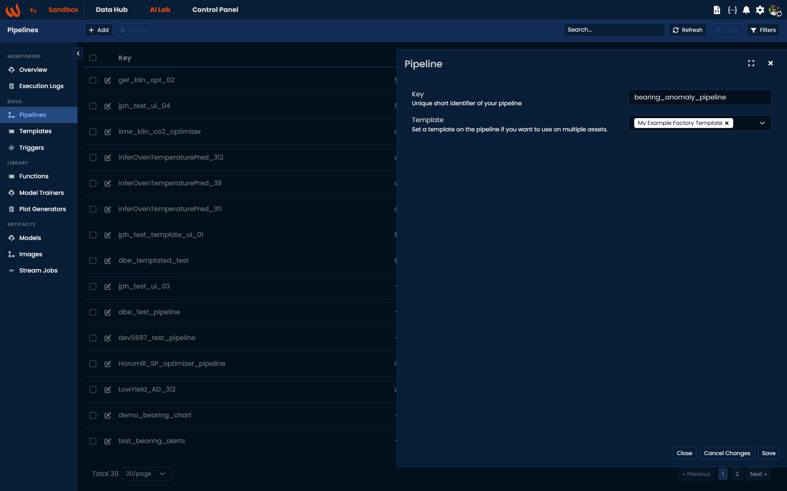
Alternatively, you can create the pipeline directly from the platform. Navigate to AI Lab → Pipelines, click + Add, set the pipeline key (e.g., bearing_anomaly_pipeline), and assign the template you created earlier (in this case, My Example Factory Template) Then click Save.
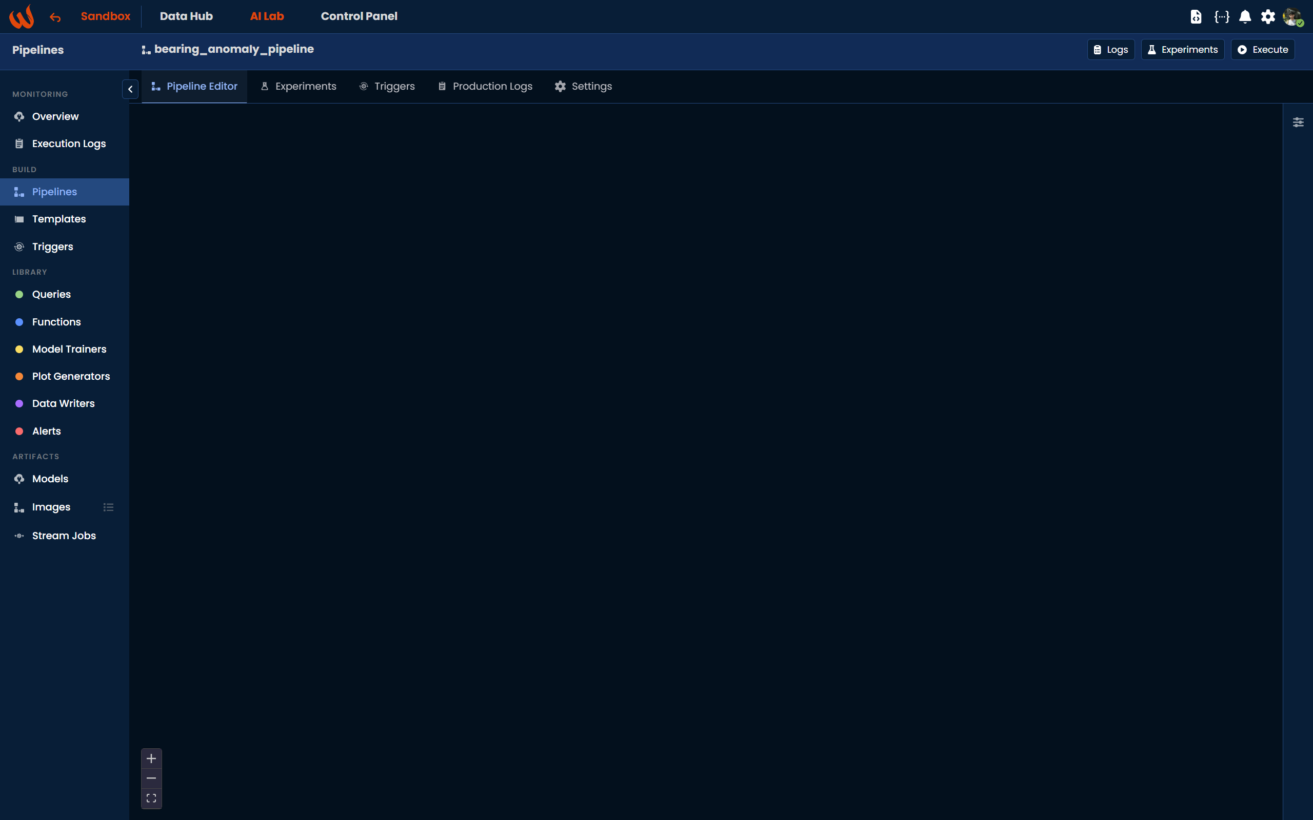
Starting from v12.0 we introduced an updated Pipeline UI that makes building your pipeline logic significantly easier. Once you save the pipeline, you are automatically redirected to the Pipeline Editor, an interactive block-based canvas where you can visually compose your solution step by step. At this point, the canvas is empty and ready for you to start building the anomaly detection logic.
In the sections below, we will walk through each step of the pipeline using both the Python Toolkit and the new Pipeline UI.
Building the query
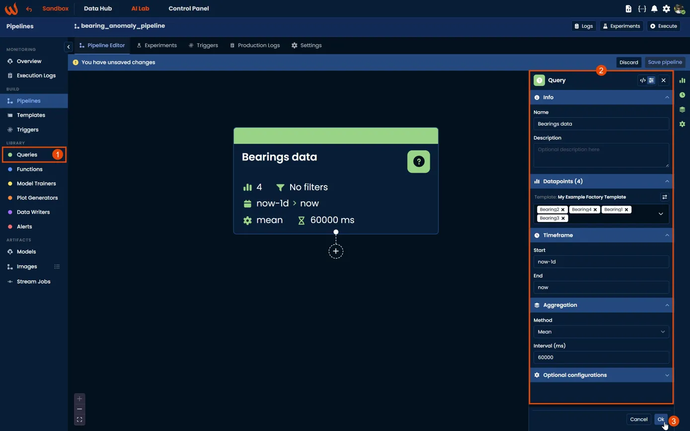
The first step for this pipeline (and most of the pipelines you will create later on) is the Query block, which is responsible for fetching the time-series data that will be processed by the subsequent steps. In this case, the query retrieves the four bearing sensor datapoints (Bearing1, Bearing2, Bearing3, and Bearing4) registered in the template earlier. These are automatically resolved to their corresponding real datapoints for each motor (Motor 1 and Motor 2) at execution time.
Using the Python Toolkit, you can define the query step as follows:
pipeline.add_query(  #query step
    wizata_dsapi.Request(
        datapoints =["Bearing1","Bearing2","Bearing3","Bearing4"],
        start="now-1d",
        end="now",
         agg_method="mean",
        interval=60000
    ),
    df_name="query_df"
)
The key parameters here are:
datapoints: the template property names already assigned to be queried.start / end: the time window to retrieve;now-1dtonowmeans the last 24 hours (you can also usenow-24h).agg_method: the aggregation method applied to the data;meanaverages the values within each interval.interval: the aggregation interval in milliseconds;60000means one data point per minute.df_name: the name given to the resulting dataframe, used to reference it in subsequent steps.
For the full list of available options, refer to the SDK Request reference.
Using the Pipeline UI, you can add a Query block in two ways:
- Drag and drop the Queries item from the left-hand Library panel onto the canvas.
- Clickon Queries in the Library panel and then click the + Create new query button that appears.
Once the block is added to the canvas, a configuration panel will open on the right side. Set the same parameters as above: select the template datapoints (Bearing1, Bearing2, Bearing3, Bearing4), define the timeframe (now-1d to now), set the aggregation method to mean and the interval to 60000 ms. When done, click Ok to confirm and save the block to the canvas.
Output Block
Once the Query block is configured, click the + button at the bottom of the block to create an output block. Name it query_df. This output block will later be connected as the input of the next step in the pipeline.
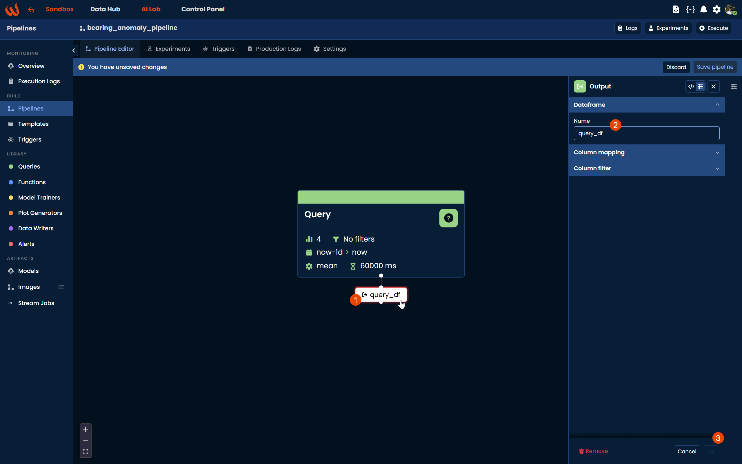
You can also click on the output block to open its configuration panel, where you can set up column mapping to rename columns before passing them to the next step, and column filters to include or exclude specific columns. This is particularly useful in templated pipelines where the query returns real datapoint names like mt1_bearing1 that need to be mapped to template property names like Bearing1 for the downstream steps. For more details, refer to the Query step article.
Designing a custom script
The next step is to create a script that preprocesses the bearing data before it is fed into the machine learning model. This transformation cleans the dataset by removing irrelevant readings, ensuring the model only trains and predicts on meaningful data. The preprocessing script does the following:
- Retrieves the dataframe from the pipeline context, which contains the data fetched by the query step.
- Drops downtimes by filtering out rows where all sensor values are below 0.05, which typically correspond to periods where the motors are not running.
- Removes null values to avoid any errors during model training or prediction.
Using the Python Toolkit, you first define and register the script on the platform, then add it as a step in the pipeline:
def bearing_preprocessing(context:wizata_dsapi.Context):
    df = context.dataframe # defines dataframes, this will come from the query step of pipeline
    df = df[(df > 0.05).any(axis=1)] # drop downtimes
    df = df.dropna() # drop null values
    return df

wizata_dsapi.api().upsert(bearing_preprocessing) # this save the transformation script into the platform pipeline.add_transformation( # script step
script="bearing_preprocessing",
input_df_names=['query_df'],
output_df_names=['df_processed']
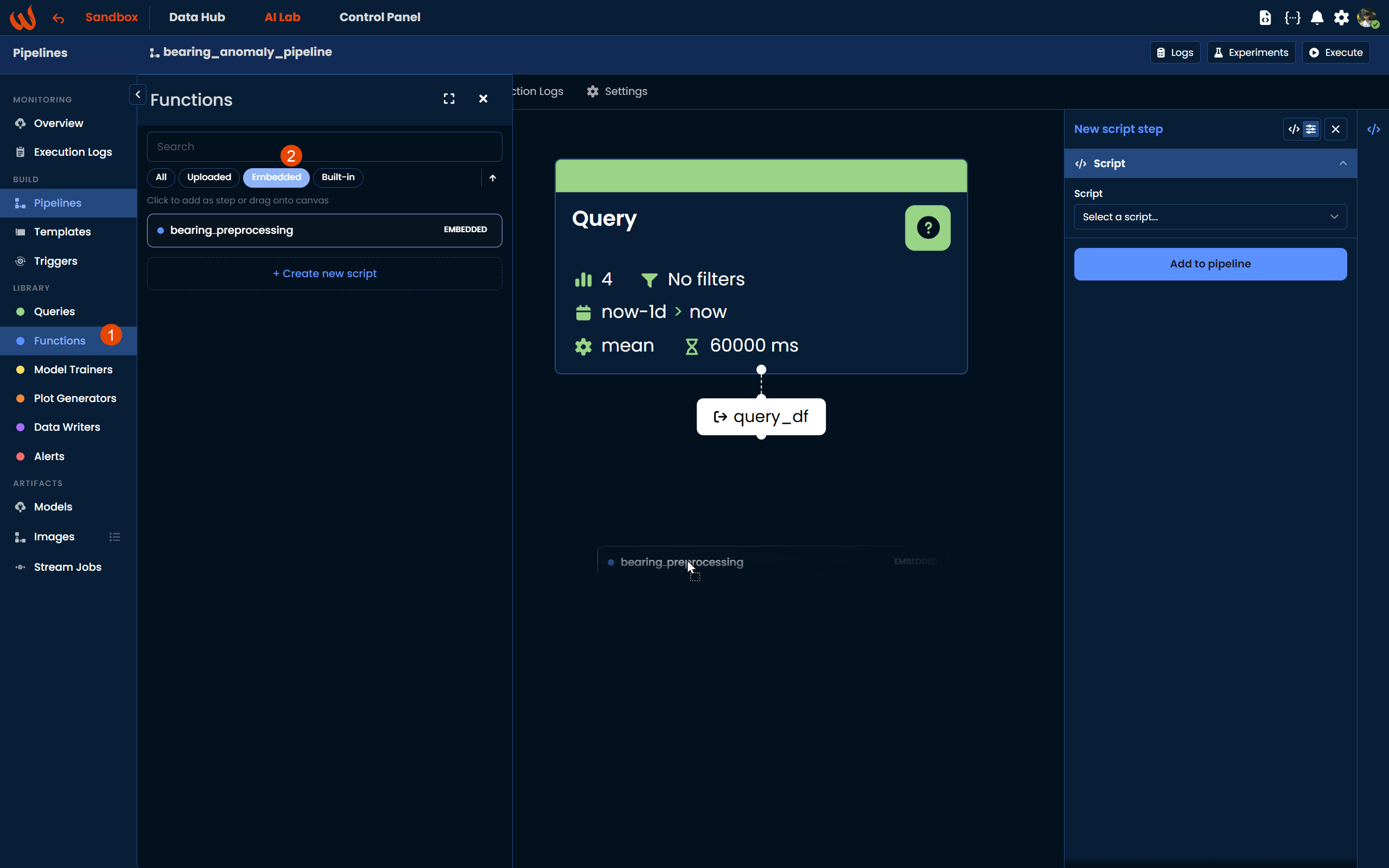
)Using the Pipeline UI, you can create the script directly from the platform. Navigate to Library > Functions, click + Create a new script, and write the preprocessing logic. Once complete, click Save. The script will then be available under Library > Functions as an Embedded script, which is the type assigned to scripts created directly from the platform.
For more information on the different script types available, refer to the Script step article.
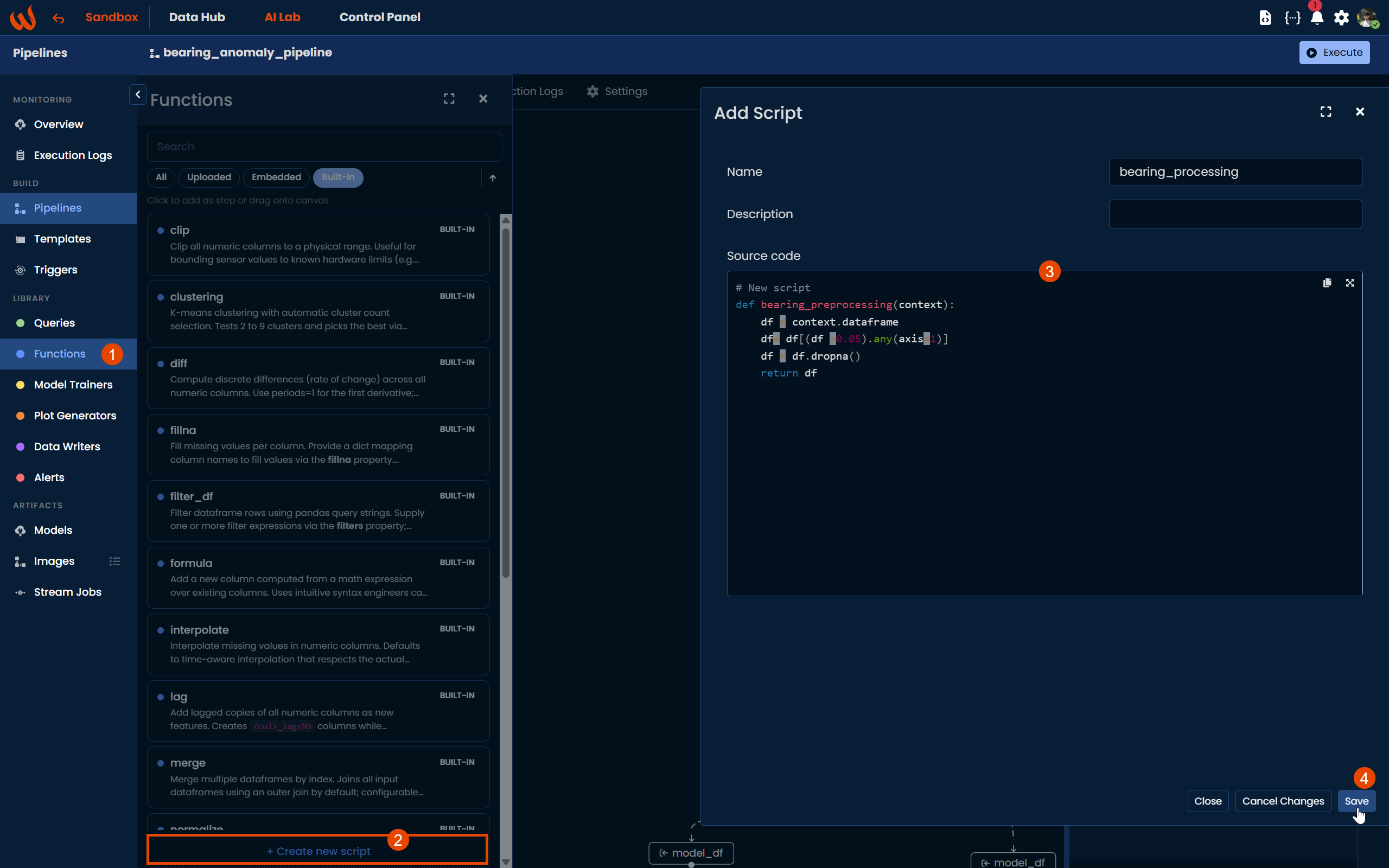
Make sure the function name in the script definition matches the name set in the form. Also, remember to include the
contextparameter in your function signature to be able to retrieve the dataframe from the Query step.
To add the script to your pipeline canvas, drag and drop it from the Embedded scripts list onto the canvas.
Connecting inputs and outputs
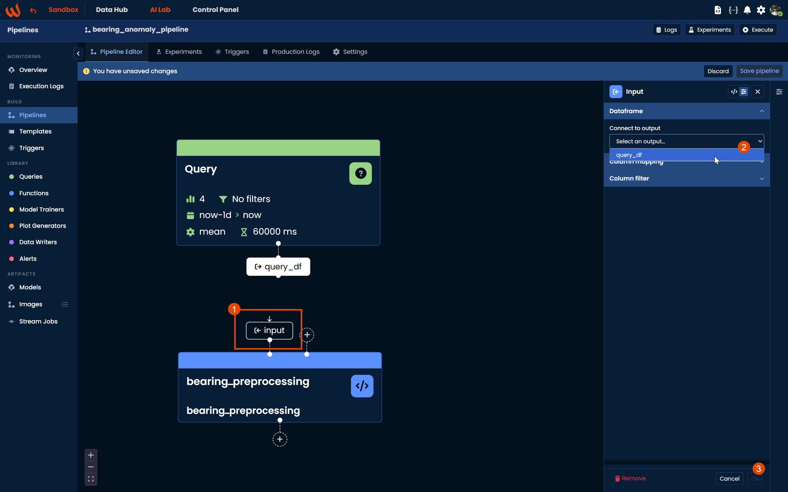
Once the script block is on the canvas, click the + button at the input side of the block. The input block will appear, and on the right-hand panel select Connect to output and enter the name of the output block you want to connect, in this case query_df, which is the output of the Query block.
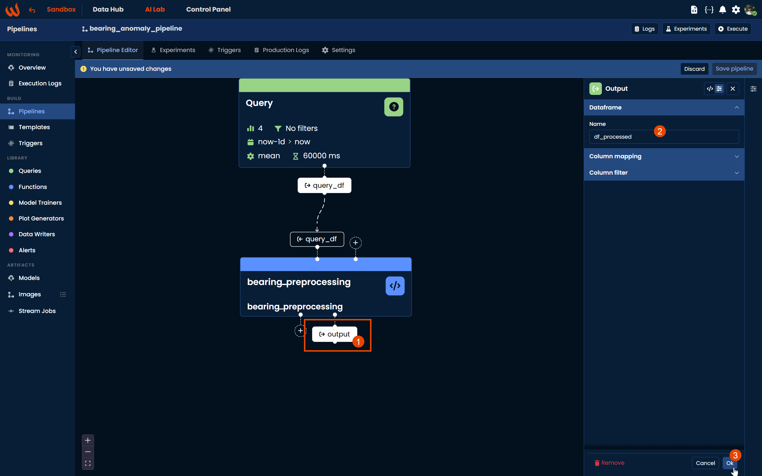
Similarly, click the + button at the output side of the script block to create an output block named df_processed. This will be used as the input of the next step, the Model block.
Configuring the model
With the preprocessed data ready, the next step is to configure the model that will be trained to detect anomalies in the bearing data. We are using an Isolation Forest, an unsupervised machine learning algorithm well suited for anomaly detection on multivariate sensor data. It works by isolating observations through random partitioning, making it effective at identifying data points that behave differently from the rest without needing labeled examples of anomalies.
There are two ways to set up the model in this tutorial: using a custom model script or using the built-in Isolation Forest available directly in the platform.
Option 1: Custom Model Script
Using the Python Toolkit, you first define and register the model training script, then configure the model step in the pipeline:
def anomaly_detection_model(context: wizata_dsapi.Context):
    df = context.dataframe
    from sklearn.ensemble import IsolationForest

    # Create and fit the model
    iso_forest = IsolationForest(contamination=0.01, random_state=42)  # Adjust contamination based on your data
    iso_forest = iso_forest.fit(df)
    context.set_model(iso_forest, df.columns)

wizata_dsapi.api().upsert(anomaly_detection_model)pipeline.add_model(
config=wizata_dsapi.MLModelConfig(
train_script='anomaly_detection_model', # this is the model script
features=["Bearing1","Bearing2","Bearing3","Bearing4"], # input features for model
output_append=True, # it will append the prediction results
output_columns_names=["bearing_anomaly"], # prediction output column's name, it will return model.predict(df["features"])
function="predict", # it can be, transform, predict etc.
model_key="ad_model", # this is the name of model as saved in the platform
by_twin=True # it will save the model seperately by twin. like ad_model_motor1,ad_model_motor1
),
input_df='df_processed',
output_df='model_df'
)
The key parameters in MLModelConfig are:
train_script: the name of the training script registered in the platform, used to fit the model during experiment runs.features: the list of input columns the model will be trained and evaluated on, referencing the template property names.output_append: when set to True, the prediction results are appended as new columns to the existing dataframe rather than replacing it.output_columns_names: the name(s) assigned to the output prediction column(s). In this case, bearing_anomaly will contain the model output.function: the method called on the trained model during production runs. Common options are predict and transform.model_key: the identifier used to store and retrieve the model in the platform.by_twin: when set to True, a separate model is saved for each twin. In this tutorial that results inad_model.motor_1andad_model.motor_2, so each motor has its own trained model without needing a separate pipeline.
For the full list of available parameters, refer to the MLModelConfig.
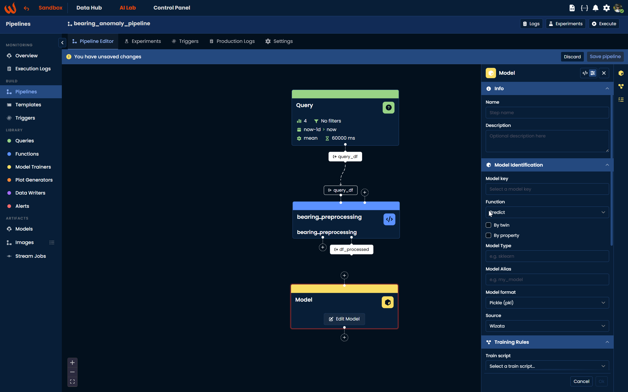
Using the Pipeline UI, you can add a Model Trainer block the same way as the previous steps: navigate to Library > Model Trainers and either drag and drop your custom model trainer onto the canvas or click + Create new model to define a new one. Once added, the configuration panel will open on the right side where you can set the same parameters described above.
Option 2: Built-in Isolation Forest
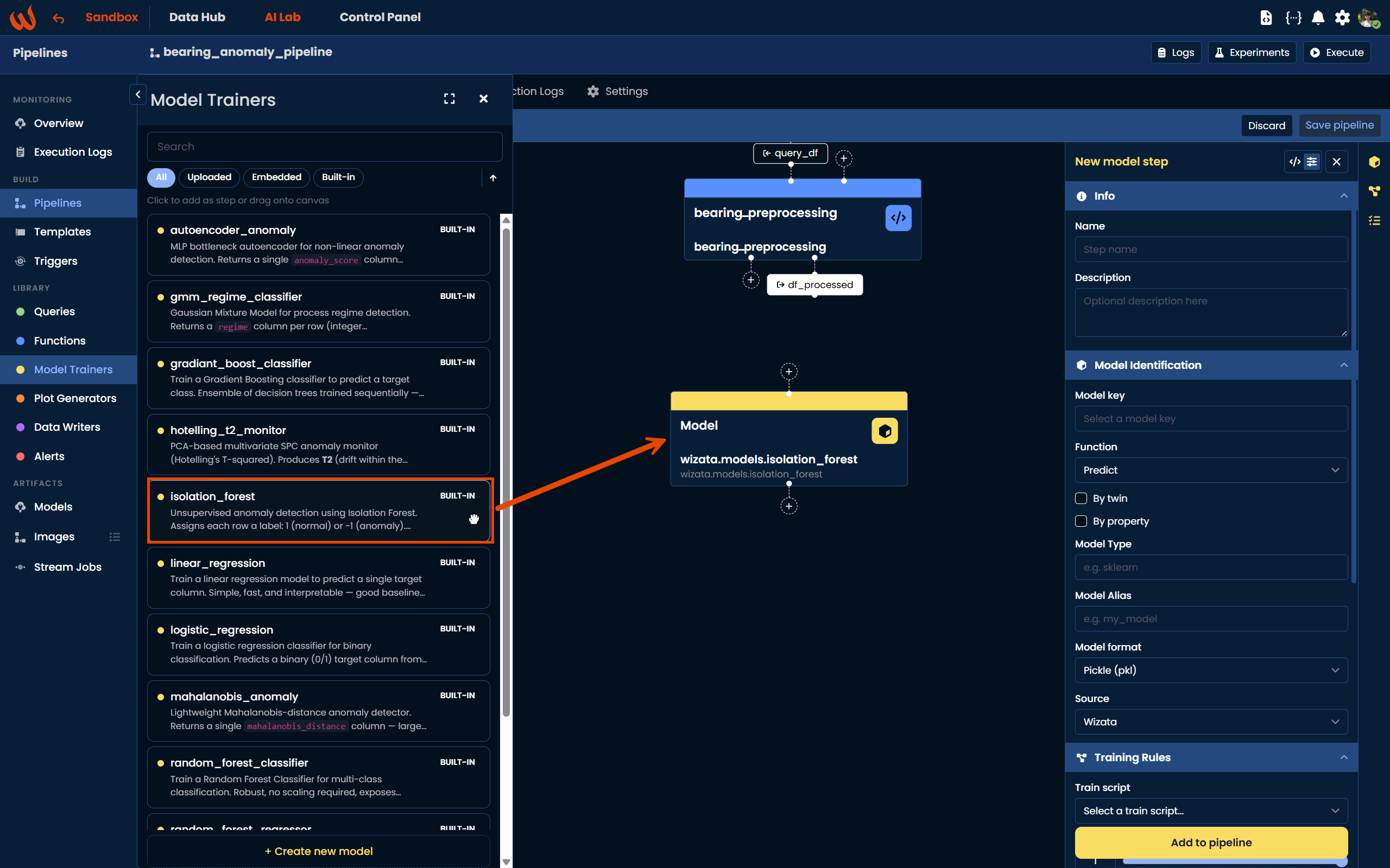
As an alternative to writing a custom script, Wizata provides a built-in Isolation Forest model trainer available directly in the Library. In the Pipeline UI, you can find it under Library > Model Trainers by filtering for Built-in models. Simply drag the isolation_forest block onto the canvas and configure the sensitivity parameter in the right-hand panel, which controls the contamination level (from 1 for few anomalies to 5 for many anomalies).
Using the Python Toolkit, the built-in model can be referenced directly by its library key:
Note that the sensitivity parameter is not part of the model configuration itself, but must be passed separately as a property. You can either hardcode it in the pipeline definition so it is applied automatically on every execution:
ml_config = wizata_dsapi.MLModelConfig(
    train_script='wizata.models.isolation_forest',
    features=["Bearing1", "Bearing2", "Bearing3", "Bearing4"],
    output_append=True,
    output_columns_names=["bearing_anomaly"],
    function="predict",
    model_key="ad_model",
    by_twin=True
)
ml_config.properties = {"sensitivity": 3}

pipeline.add_model(
    config=ml_config,
    input_df='df_processed',
    output_df='model_df'
)
Or you can pass it at runtime when executing the experiment or deploying the pipeline, without modifying the pipeline definition. We will cover this in detail in the Testing and Deploying the Pipeline section below.
For more details on the available built-in functions and model trainers, refer to the Wizata library for common functions
Model Output
Regardless of which approach you choose, after the model step the output dataframe model_df will contain the original bearing columns plus the prediction result: ["Bearing1", "Bearing2", "Bearing3", "Bearing4", "bearing_anomaly"].
As with the previous steps, create an output block by clicking the + button at the bottom of the Model block and name it model_df. This will be used as the input for the next step.
Visualizing the Results
To inspect the model output during experimentation, we can add a plot step to the pipeline. This step is intended for experiment runs only and will not execute in production. It allows you to visually verify that the anomaly detection is working as expected before deploying the pipeline. Similarly to the model step, there are two approaches: writing a custom plot script or using a built-in plot from the Wizata library.
Option 1: Custom Plot Script
The custom script creates a line chart of the bearing sensor values and marks detected anomalies with red vertical lines. The bearing_anomaly column, which contains -1 for anomalies and 1 for normal readings, is used to identify where to place those markers. Using the Python Toolkit, register the plot script and add it to the pipeline:
def bearing_ad_plot(context: wizata_dsapi.Context):
    df = context.dataframe
    import plotly.graph_objects as go

    # Create the line plot
    fig = go.Figure()

    # Add traces for each sensor
    for column in df.columns[1:-1]:  # Exclude the 'Timestamp' and 'anomaly' columns
        fig.add_trace(go.Scatter(x=df.index, y=df[column], mode='lines', name=column))

    # Add vertical lines for anomalies
    anomaly_times = df[df['bearing_anomaly'] == -1].index
    for anomaly_time in anomaly_times:
        fig.add_vline(x=anomaly_time, line=dict(color='red', width=2))

    # Update layout
    fig.update_layout(
        title="Sensor Data with Anomaly Detection",
        xaxis_title="Timestamp",
        yaxis_title="Sensor Values",
        showlegend=True
    )

    context.set_plot(fig, "Bearing Anomaly Detection")  # save with the title

wizata_dsapi.api().upsert(bearing_ad_plot)pipeline.add_plot(df_name="model_df", script="bearing_ad_plot") # plot stepUsing the Pipeline UI, navigate to Library > Plot Generators, drag your custom plot script onto the canvas and connect model_df as its input, following the same steps described in the previous sections.
Option 2: Built-in Anomaly Chart
As an alternative, Wizata provides a built-in plot generator called wizata.plots.anomalies_chart, designed specifically for visualizing anomaly detection results. In the Pipeline UI, you can find it under Library > Plot Generators by filtering for Built-in plots and dragging it onto the canvas.
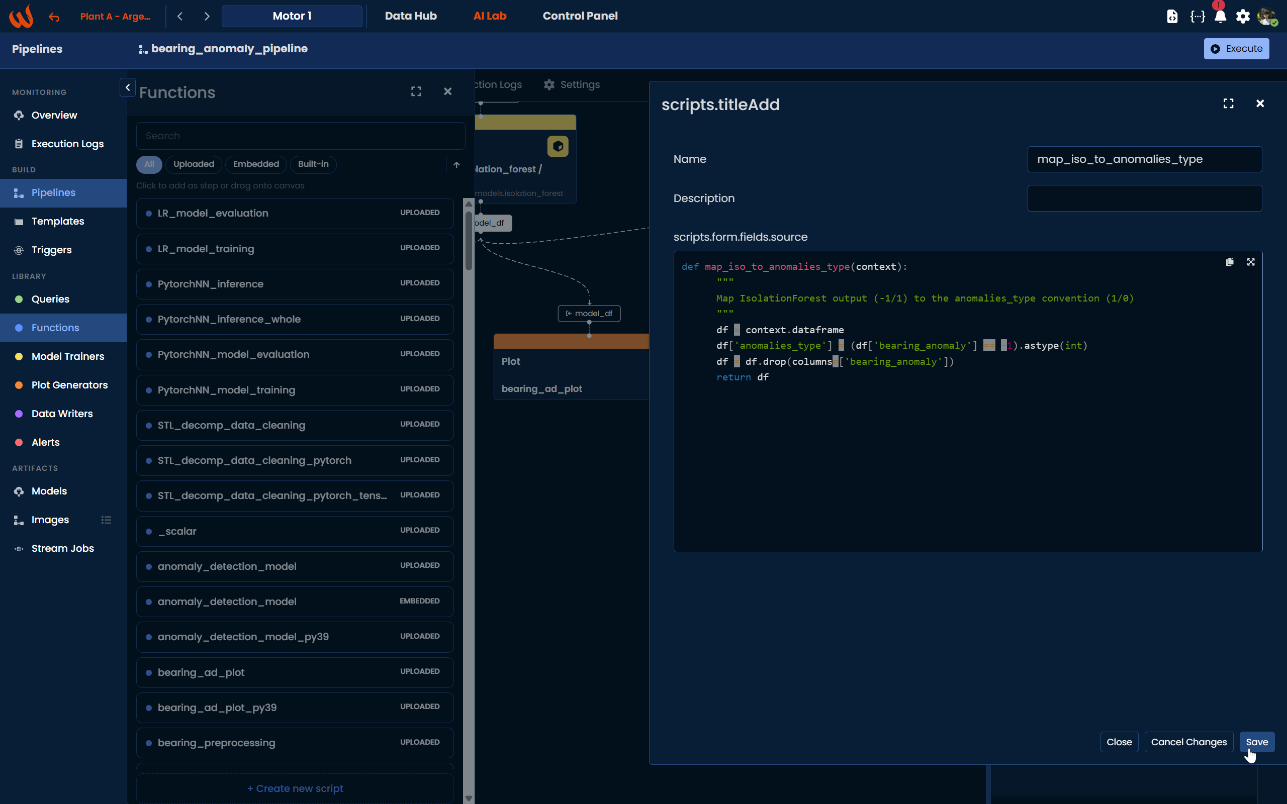
Before connecting the plot, there is one important step to add: the built-in anomalies_chart expects a column named anomalies_type where 0 means normal and any non-zero value means anomaly. The built-in Isolation Forest model, however, outputs the raw scikit-learn values (-1 for anomalies, 1 for normals) under the column name set in the model block (bearing_anomaly in our case). To bridge the two, a small transformation script is needed between the model and the plot.
Using the Python Toolkit, register the mapping script and add it as a step between the model and the plot:
def map_iso_to_anomalies_type(context):
    df = context.dataframe
    df['anomalies_type'] = (df['bearing_anomaly'] == -1).astype(int)
    df = df.drop(columns=['bearing_anomaly'])
    return df

wizata_dsapi.api().upsert(map_iso_to_anomalies_type)

pipeline.add_transformation(
    script="map_iso_to_anomalies_type",
    input_df_names=["model_df"],
    output_df_names=["df_anomalies"]
)

pipeline.add_plot(df_name="df_anomalies", script="wizata.plots.anomalies_chart")
Using the Pipeline UI, navigate to Library > Functions and create the mapping script using the + Create new script button. Once saved, drag a Script block onto the canvas between the Model block and the Plot block. Connect the model's output dataframe (model_df) as the script input, and the script's output (df_anomalies) as the input of the built-in anomaly chart plot block.
In this tutorial we will use both, so you can compare the outputs side by side when running the pipeline in experiment mode.
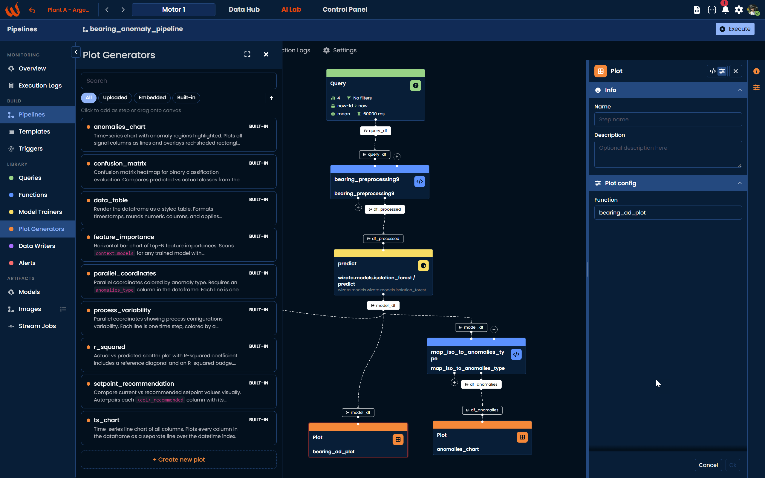
The plot step only runs during experiment executions. Once you run the pipeline as an experiment, the generated charts will be available in the Experiments tab of the pipeline. For more details on built-in plot generators, refer to the Wizata library for common functions
Writing the Results
The final step is to write the model output back to the platform. In this case, we want to store the bearing_anomaly column so that the anomaly detection results are available as a datapoint that can be monitored, visualized, or used to trigger alerts. Using the Python Toolkit, add the writer step as follows:
pipeline.add_writer( #writer step
    config=wizata_dsapi.WriteConfig(
        datapoints={
            "bearing_anomaly":"bearing_anomaly"
        }
    ),
    input_df='model_df'
)
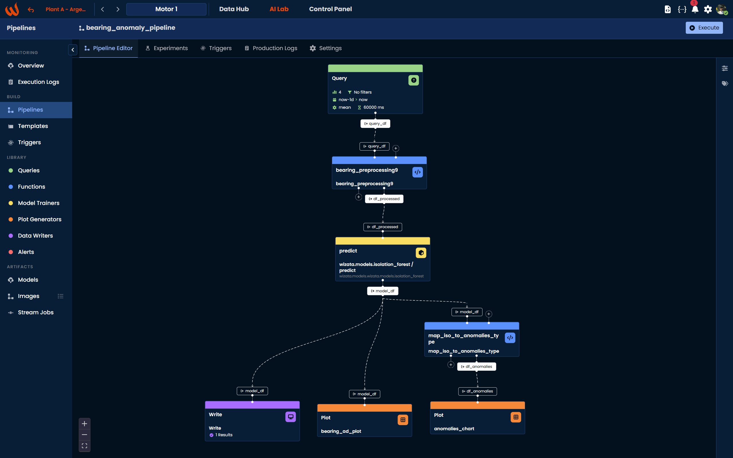
The mapping in datapoints follows the format {"output_column": "template_property"}. In this case, the bearing_anomaly column produced by the model step is written to the bearing_anomaly template property registered earlier, which resolves to the actual datapoint for each twin at execution time.
Using the Pipeline UI, drag the Data Writers block from the Library panel onto the canvas and connect model_df as its input. In the configuration panel, set up the same mapping: assign the bearing_anomaly output column to the bearing_anomaly template property. That is all the configuration needed for this use case.
(NEW) Setting Up Anomaly Alerts
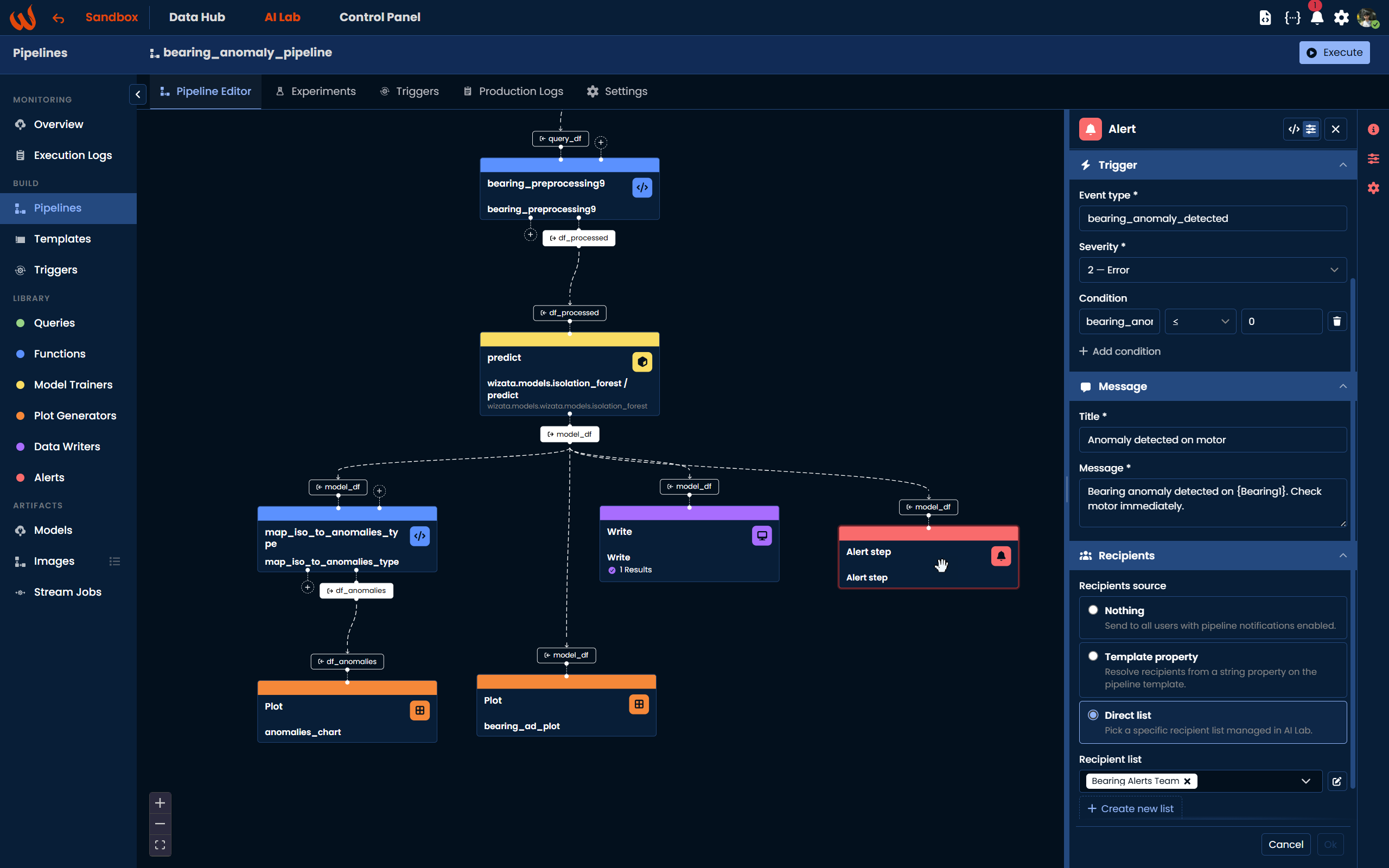
With the pipeline running in production and detecting anomalies in real time, the next natural step is to receive a notification whenever an anomaly is detected on a motor. For this, we add an Alert block connected to the output of the model step (model_df).
Creating a Recipient List
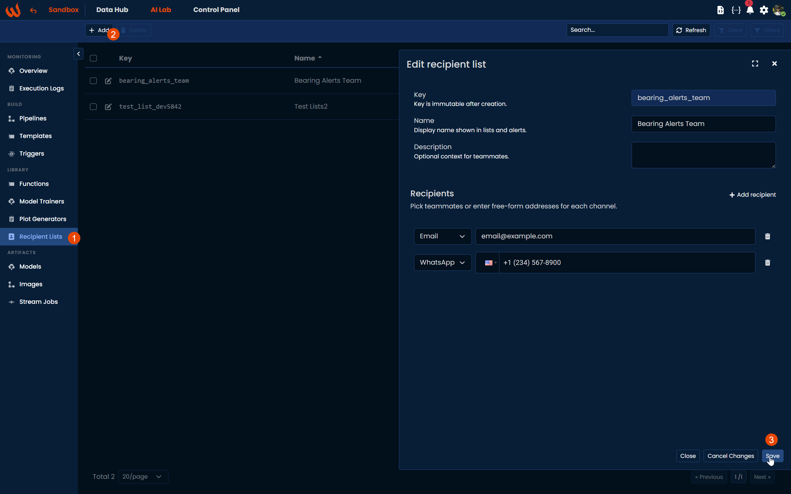
Before configuring the Alert block, you can optionally create a Recipient List to define who should be notified. Navigate to AI Lab > Library > Recipient Lists and click + Add. Set a key such as bearing_alerts_team and a display name like "Bearing Alerts Team". Then add the recipients, typically the maintenance engineers responsible for the motors.
Adding the Alert Block
The Alert block evaluates a condition against the first row of the input dataframe on each pipeline execution. In our case, the bearing_anomaly column contains -1 when an anomaly is detected and 1 for normal readings. We configure the condition to fire when that value is less than or equal to 0, which covers the anomaly case.
Using the Pipeline UI, navigate to Library > Alerts in the left-hand panel and drag the block onto the canvas. Connect model_df as its input. In the configuration panel, set the following:
- Event type:
bearing_anomaly_detected - Severity: 2 (Error)
- Condition:
bearing_anomalyless than or equal to0 - Title:
Anomaly detected on motor - Message:
Bearing anomaly detected on {Bearing1}. Check motor immediately. - Recipients: select the
bearing_alerts_teamlist created earlier - Activation threshold:
2(require 2 consecutive detections before notifying, to avoid false positives) - Expiration cycles:
3(the episode closes if 3 consecutive executions show no anomaly)
Using the Python Toolkit, add the alert step as follows:
alert_cfg = wizata_dsapi.AlertConfig(
    mode="declarative",
    event_type="bearing_anomaly_detected",
    severity=2,                               # Error severity
    title="Anomaly detected on motor",
    message="Bearing anomaly detected. Check motor immediately.",
    condition={
        "bearing_anomaly": {"lte": 0}         # fires when bearing_anomaly == -1
    },
    recipient_list_key="bearing_alerts_team", # the recipient list created earlier
    activation_threshold=2,                   # require 2 consecutive hits before notifying
    expiration_cycles=3,                      # episode closes after 3 missed intervals
    channels=[wizata_dsapi.AlertType.PUSH_NOTIFICATION, wizata_dsapi.AlertType.EMAIL]
)

pipeline.add_alert(
    config=alert_cfg,
    df_name="model_df"
)
The Alert step takes one input and produces no output. It must be the last block connected to the model output in the pipeline. For more details on all available configuration options, refer to the Alert step article.
Next steps
Once the writer block is saved, the pipeline is complete. Click Save pipeline at the top of the canvas to persist all the changes before moving on to testing and deployment.
If you have been following the Python Toolkit approach, once all steps are defined the final action is to upsert the pipeline to the platform:
wizata_dsapi.api().upsert_pipeline(pipeline)Below is the complete pipeline script for reference:
import uuid

# Generate pipeline
pipeline = wizata_dsapi.Pipeline(
    key="bearing_anomaly_pipeline",
    template_id=uuid.UUID("61d63f8b-6142-43bc-bb98-ac146076601b")  # template id from the template link
)

pipeline.add_query(  # query step
    wizata_dsapi.Request(
        datapoints=["Bearing1", "Bearing2", "Bearing3", "Bearing4"],
        start="now-1d",
        end="now",
        agg_method="mean",
        interval=60000,
    ),
    df_name="query_df"
)

pipeline.add_transformation(  # preprocessing script step
    script="bearing_preprocessing",
    input_df_names=['query_df'],
    output_df_names=['df_processed']
)

pipeline.add_model(
    config=wizata_dsapi.MLModelConfig(
        train_script='anomaly_detection_model',
        features=["Bearing1", "Bearing2", "Bearing3", "Bearing4"],
        output_append=True,
        output_columns_names=["bearing_anomaly"],
        function="predict",
        model_key="ad_model",
        by_twin=True  # saves the model separately per twin: ad_model.motor_1, ad_model.motor_2
    ),
    input_df='df_processed',
    output_df='model_df'
)

pipeline.add_plot(df_name="model_df", script="bearing_ad_plot")  # custom plot step

pipeline.add_writer(  # writer step
    config=wizata_dsapi.WriteConfig(
        datapoints={
            "bearing_anomaly": "bearing_anomaly"
        }
    ),
    input_df='model_df'
)

wizata_dsapi.api().upsert_pipeline(pipeline)
import uuid
# Generate pipeline
pipeline = wizata_dsapi.Pipeline(
key="bearing_anomaly_pipeline",
template_id=uuid.UUID("61d63f8b-6142-43bc-bb98-ac146076601b") # template id from the template link
)
pipeline.add_query( # query step
wizata_dsapi.Request(
datapoints=["Bearing1", "Bearing2", "Bearing3", "Bearing4"],
start="now-1d",
end="now",
agg_method="mean",
interval=60000,
),
df_name="query_df"
)
pipeline.add_transformation( # preprocessing script step
script="bearing_preprocessing",
input_df_names=['query_df'],
output_df_names=['df_processed']
)
# Built-in Isolation Forest model
ml_config = wizata_dsapi.MLModelConfig(
train_script='wizata.models.isolation_forest',
features=["Bearing1", "Bearing2", "Bearing3", "Bearing4"],
output_append=True,
output_columns_names=["bearing_anomaly"],
function="predict",
model_key="ad_model",
by_twin=True # saves the model separately per twin: ad_model.motor_1, ad_model.motor_2
)
ml_config.properties = {"sensitivity": 3} # hardcoded sensitivity, alternatively pass at runtime
pipeline.add_model(
config=ml_config,
input_df='df_processed',
output_df='df_predict'
)
# Mapping step: convert isolation forest output (-1/1) to anomalies_type format (0/1)
pipeline.add_transformation(
script="map_iso_to_anomalies_type",
input_df_names=["df_predict"],
output_df_names=["df_anomalies"]
)
pipeline.add_plot(df_name="df_anomalies", script="wizata.plots.anomalies_chart") # built-in plot step
pipeline.add_writer( # writer step
config=wizata_dsapi.WriteConfig(
datapoints={
"bearing_anomaly": "bearing_anomaly"
}
),
input_df='df_predict' # write from df_predict, before the mapping step
)
wizata_dsapi.api().upsert_pipeline(pipeline)Testing and Deploying the Pipeline
After having the pipeline in the platform, the next step is to test whether it runs correctly. To do this, we will run the pipeline in Experiment mode. There are two ways to run a pipeline: Experiment mode and Production mode. The difference between them is as follows:
- Experiment mode: This mode is essentially for testing whether the pipeline runs correctly. By default, the write step is not executed in this mode. The pipeline goes through the query, transformation, model, and plot steps, and the experiment returns a plot to verify that the pipeline is functioning properly.
- Production mode: This mode is used to run the pipeline in real-time. In production mode, the write step is executed, and the key difference is that the model step uses a pre-trained model for prediction rather than training a new model. At the end of the process, the results are written to the platform.
In summary, you should first run the pipeline in Experiment mode to train the model, save it, and view the plot results. After that, you can run the pipeline in Production mode to make predictions and write the output to the platform.
Testing the Pipeline
Now, we will run the pipeline in Experiment mode for testing. This will train the model and return the plot as part of the experiment results. Using the Python Toolkit, create an experiment and execute the pipeline as follows:
wizata_dsapi.api().upsert_experiment("bearing_anomaly_experiment", "Bearing Anomaly Experiment", pipeline="bearing_anomaly_pipeline")

execution = wizata_dsapi.api().experiment(
    experiment='bearing_anomaly_experiment',
    pipeline='bearing_anomaly_pipeline',
    twin='motor_1'
)
wizata_dsapi.api().upsert_experiment("bearing_anomaly_experiment", "Bearing Anomaly Experiment", pipeline="bearing_anomaly_pipeline")
execution = wizata_dsapi.api().experiment(
experiment='bearing_anomaly_experiment',
pipeline='bearing_anomaly_pipeline',
twin='motor_1',
properties={"sensitivity": 3}
)If you are using the built-in Isolation Forest model and configured your pipeline using the Python Toolkit, make sure to pass the
sensitivityparameter in thepropertiesfield. This controls the contamination level of the model and must be provided at execution time if not hardcoded in the pipeline configuration.
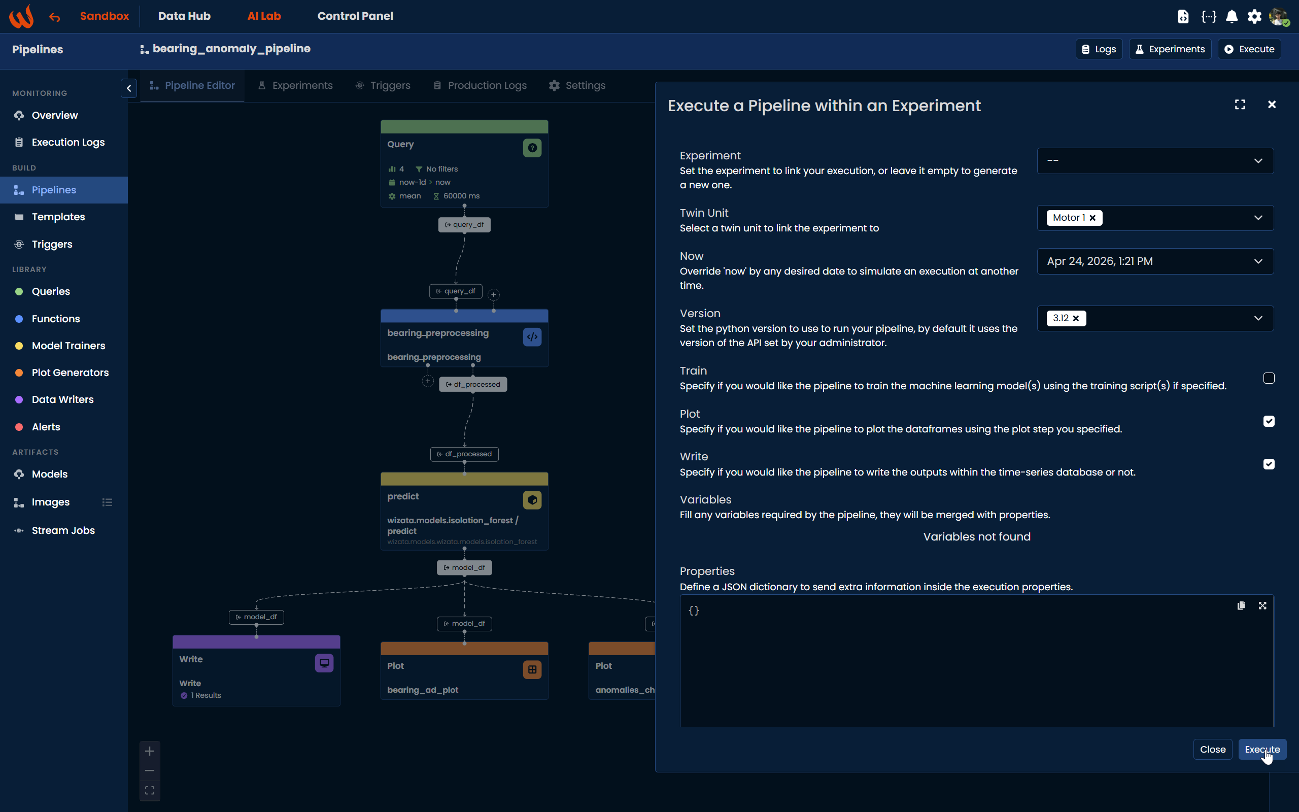
Using the Pipeline UI, click the Execute button at the top right of the pipeline. A dialog will open where you can configure the execution: select the twin unit (e.g., Motor 1), set the reference time for now, choose the Python version, and toggle whether you want to Train the model, generate the Plot, and Write the results. Once configured, click Execute to run.
Once the execution completes, navigate to the Experiments tab to see the results. Click the eye icon next to a completed execution to open the experiment detail panel on the right, where you will find the generated plots along with a summary table.
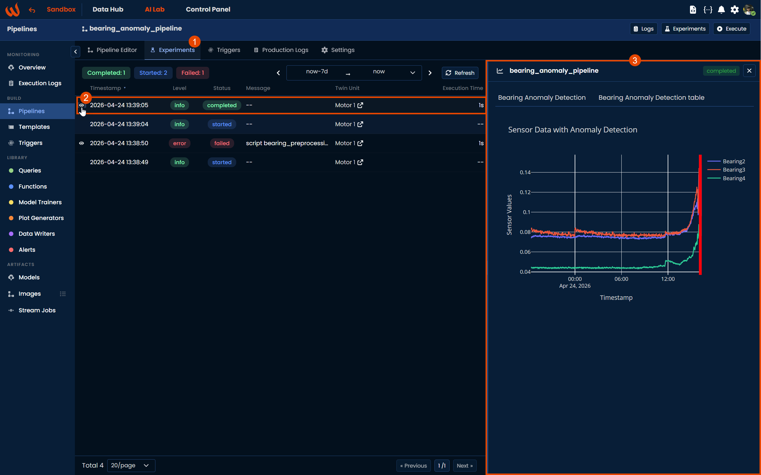
This means the pipeline ran successfully, trained the model, and saved it within the platform. We are ready to deploy the model in real time.
Deploy the Pipeline
Running the pipeline in production is two different things, and it is worth being clear which you want.
Running it once executes it now, against one twin:
production_mode = wizata_dsapi.api().run(
    pipeline='bearing_anomaly_pipeline',
    twin='motor_2')
Deploying it puts it on a schedule. That is what real-time monitoring needs: the pipeline runs every few minutes, on every motor, without anyone starting it. Deploying also publishes your draft and freezes the version that will run, so what is monitoring your bearings in six months is the code you approved today — see Deployment for the whole sequence.
From the pipeline, choose Deploy. The wizard asks where each motor should run:
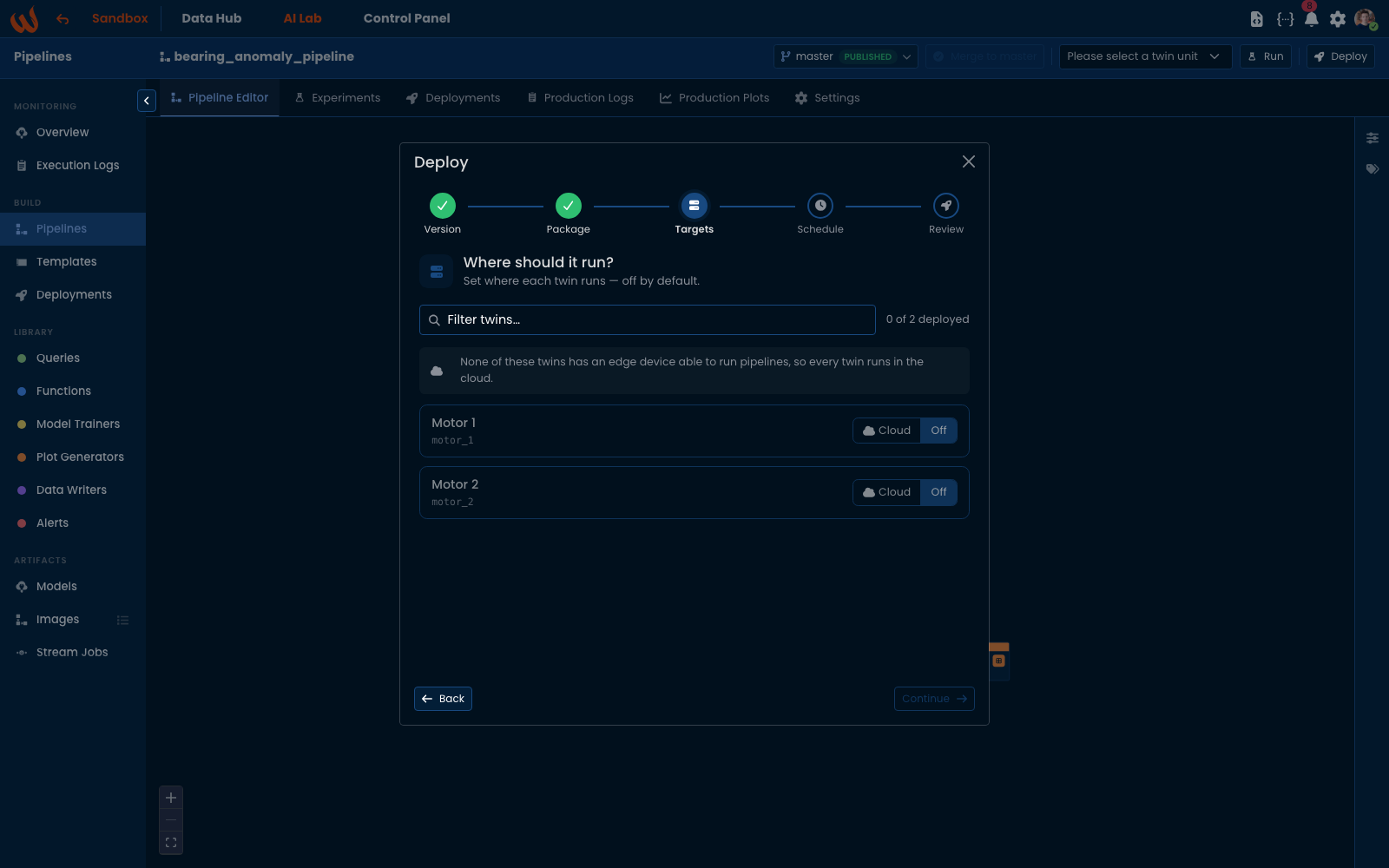
Both motors start Off — a deployment covers the twins you choose. Here neither has an edge device able to run pipelines, so both run in the cloud and the dialog says so; on a site with a capable device, an Edge option appears per twin.
Then the schedule, and what each run does:
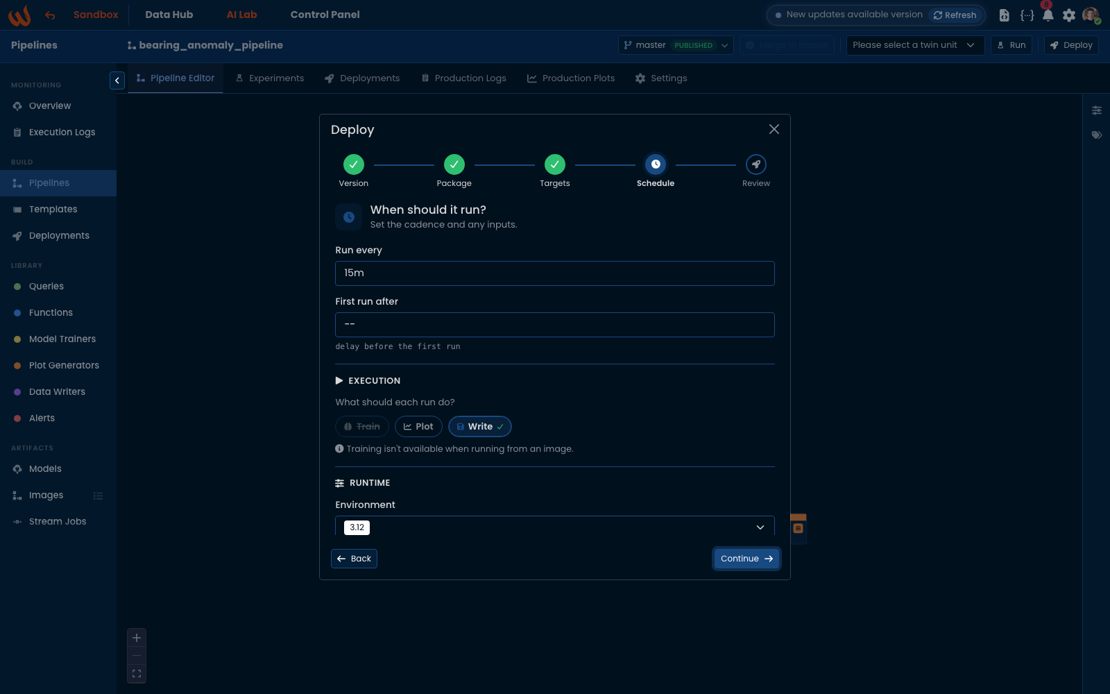
Write is on by default, which is what stores each bearing_anomaly result back as a datapoint. Train is unavailable when running from an image: the image carries the model you trained above, and that frozen model is what predict uses.
The same thing from the Python Toolkit:
deployment = wizata_dsapi.api().deploy(
    'bearing_anomaly_pipeline',
    twins=['motor_1', 'motor_2'],
    interval=300000,                       # every 5 minutes
    properties={'sensitivity': 0.05}
)

deployment = wizata_dsapi.api().await_deployment(deployment)
print(deployment.status)
If you are using the built-in Isolation Forest model and configured your pipeline using the Python Toolkit, pass
sensitivityin the deployment's properties, as above — every scheduled run receives it.If you configured the pipeline from the Pipeline UI, the sensitivity value set in the model configuration panel is saved automatically and no additional action is needed.
The dialog reads5m, the toolkit takes millisecondsThey describe the same schedule:
5misinterval=300000.
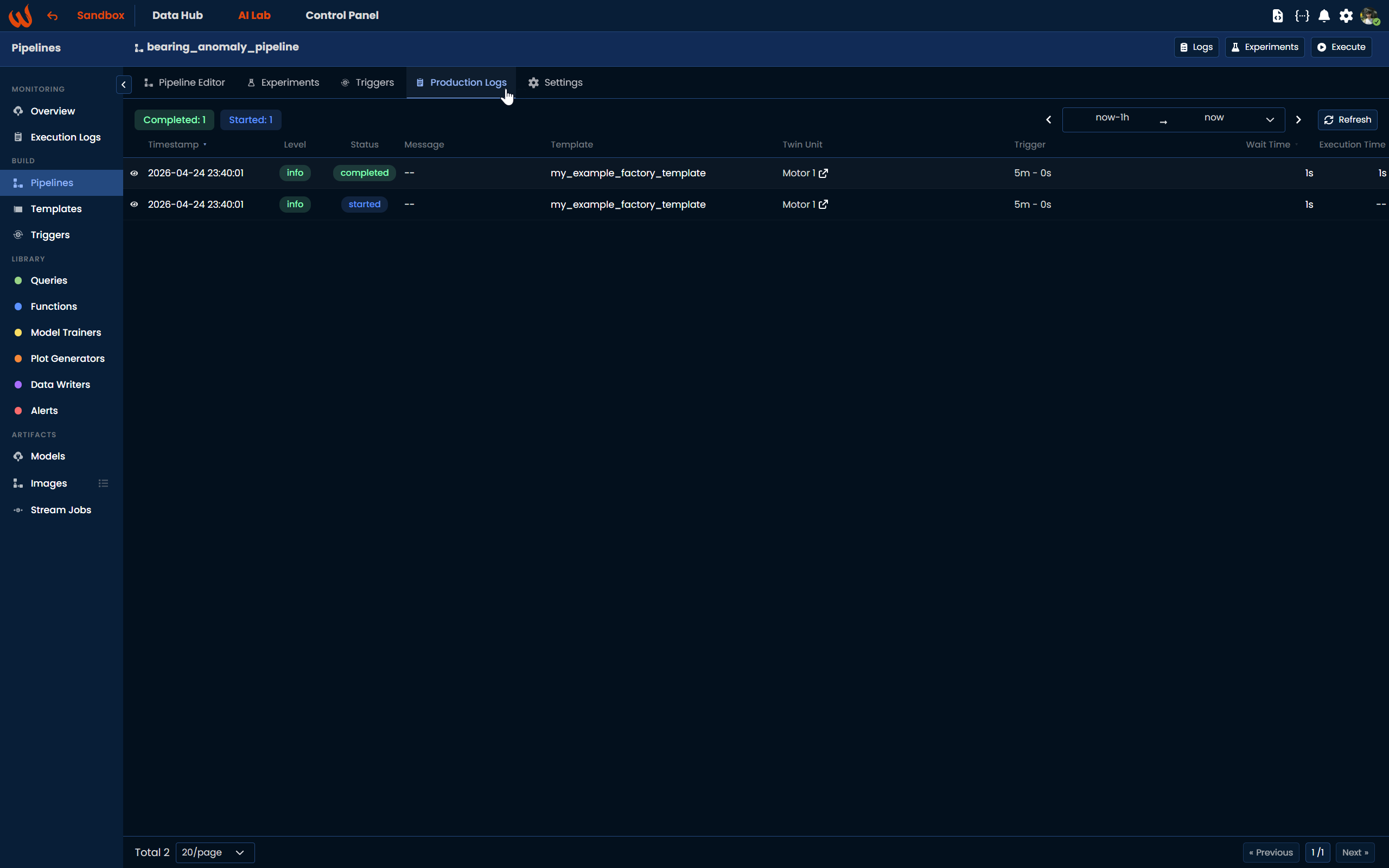
In the scenario described above, the pipeline is scheduled to run every 5 minutes for both Motor 1 and Motor 2. After this step, we can review the execution results to verify whether the pipeline is running properly for both Motor 1 and Motor 2. For this step, you should check the Execution logs page, or the Production Logs detailed for the specific pipeline.
Conclusion
In conclusion, we have successfully developed an end-to-end anomaly detection model, demonstrating each step of the process. This included creating a template, building a pipeline, and running the pipeline in real-time.
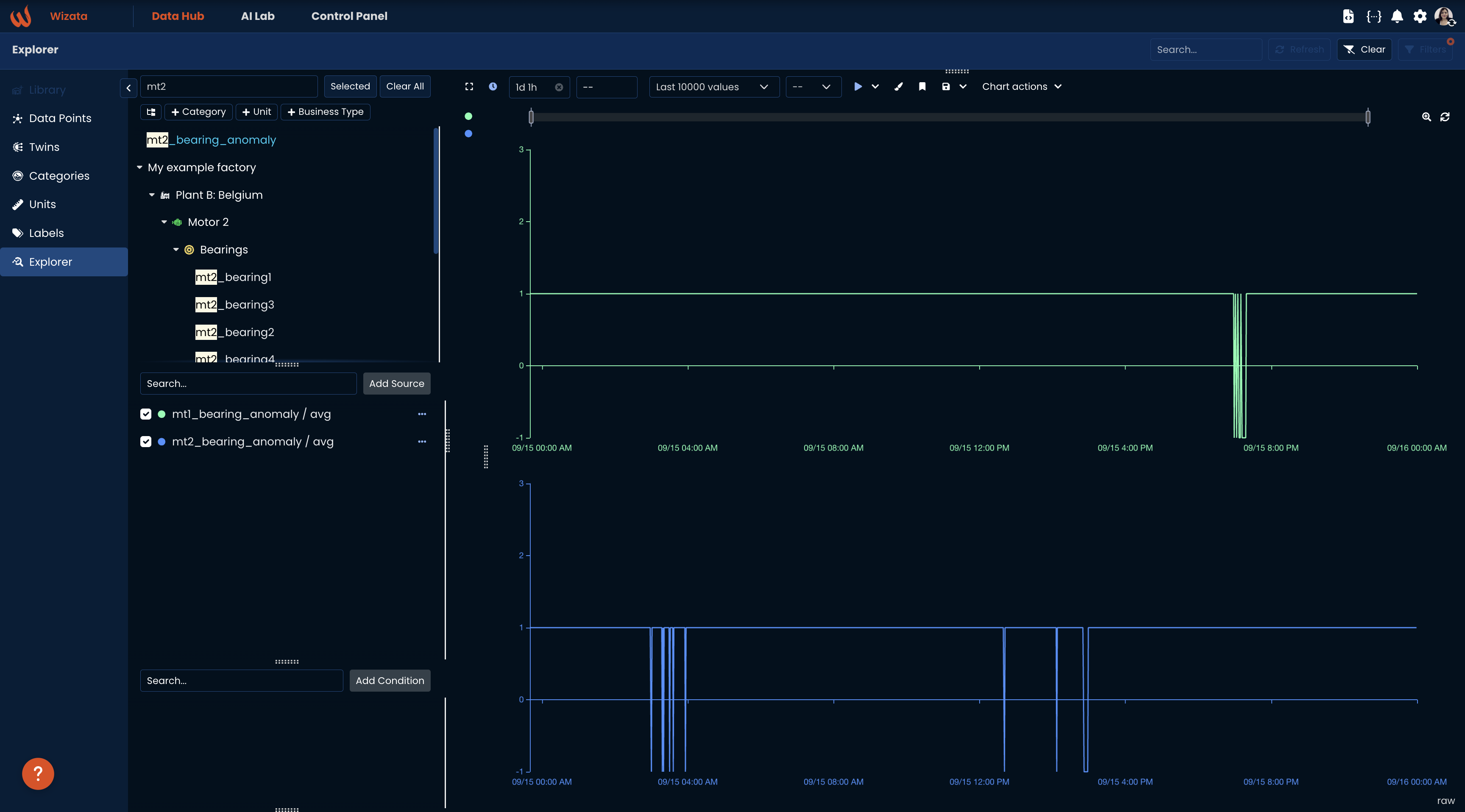
By leveraging the template, we efficiently applied the anomaly detection model to both motors, collecting the anomaly_bearing datapoints. This streamlined approach ensures that the same pipeline can be used for multiple assets, allowing for real-time monitoring and detection of anomalies across both Motor 1and Motor 2.
You can check out the bearing_anomaly outputs with the unique datapoint names in the explorer:
Updated about 1 month ago